Selection of an Appropriate Spatial Operation is Crucial in Spatial Science

When someone starts working with climate change-related task – using global or regional climate models – often one needs to perform ‘bias correction’. A bias correction process of a modelled dataset becomes quite tricky when reference dataset possesses different grid cell dimensions.  In such a scenario, the reference dataset grid is commonly rescaled to source grid i.e. Global Climate Model (GCM) or Regional Climate Model (RCM) grid. For instance, in figure (i), Grid-A is a reference grid which contains (say observed) precipitation values in millimetres (mm). While Grid-B is a source dataset (say it a modelled historic precipitation dataset). As multiple grid cells of Grid-A are falling (fully or partially) inside each of the cells of Grid-B, therefore, averaging is required to work out a single value for every cell of Grid-B. However, a standard averaging method would not work here, as different cells of Grid-A are contributing differently (area fraction-wise) to cells of Grid-B. Therefore, what we need is a ‘weighted average’ or more appropriately an ‘area-weighted average’.

Let us consider the most upper-left cell of Grid-B. As figure (ii) shows, overall, nine cells of Grid-A are contributing to this Grid-B cell. To calculate the area-weighted average (A_wAvg), first, we need to calculate contribution ratio i.e. how much area of each of the Grid-A cell is contributing to Grid-B cell. We can also call it area-weight (w). If ‘A’ is the total area of any of Grid-A cell and ‘a’ is the fractional area of that specific cell contributing to Grid-B cell, then the area-weight is given as

w = a/A

First, area weight is calculated for each of the Grid-A cells and then it is multiplied with respective grid cell value i.e. precipitation (mm). Finally, newly calculated values are summed up and divided by sum of all weights to get an area-weighted average.

Let us find the area-weighted average for Grid-B cell in figure (ii)

A_wAvg = [(363/680)×22.3 + (475.5/680)×19.5 + (82.5/680)×15.8 + (524.7/680)×27 + (680/680)×21.4 + (68.8/680)×17.2 + (1.1/680)×24.5 + (38.5/680)×20.2 + (3/680)×14.5] / [(363/680) + (475.5/680) + (82.5/680) + (524.7/680) + (680/680) + (68.8/680) + (1.1/680) + (38.5/680) + (3/680)] = 22.1 mm

Standard average = (22.3 + 19.5 + 15.8 + 27+ 21.4+ 17.2+ 24.5 + 20.2 + 14.5)/9 = 20.3 mm

There is a considerable underestimation of 1.8 mm by the standard averaging method. Even if we ignore very slightly contributing cells to calculate a standard average (20.5 mm), the difference is 1.6 mm, which is still considerable.   

In conclusion, the selection of an appropriate spatial method is very important in spatial analysis. A little negligence in selection of a method can lead to substantial inaccuracies in the final results.

Standardization of datasets preparation processes for validation of satellite-based precipitation products

Typically, the accuracy of satellite-based rainfall products is assessed using categorical and continuous statistical validation techniques. More or less these statistical techniques are quite standardized. Researchers may compare the results of various studies through common validation indices. However, there exists a major concern over datasets preparation for validation purpose. Data preparation is somewhat an unnarrated or vaguely described section in most of the research methodologies. If different researchers use different steps to prepare the same dataset for validation, then the question can be raised on their results comparison in spite of using the same validation indices. For instance, TMPA precipitation product contains hourly rain rates at every 3-hour time interval. Now, these rain rates can be compared with in-situ rainfall in two ways, i.e., comparing instantaneous rainfall rate at a specific time slot or relating 3-hourly averaged rainfall rates of in-situ data with TMPA dataset. In my perception, both techniques should provide different results, and such results are not comparable. This is just an example; some other steps are also involved in data preparation like how to take precipitation averages, how to calculate correlation coefficients (should it be calculated for rainy days only or false alarms and misses should also be included) and many more. In context to above all, I think there is a dire need to standardize processes for datasets preparation before validation.

Note: I am quite new and currently learning validation processes. If standardized processes for dataset preparation already exist then kindly guide me for those steps.

Default Projection for GIS Datsets

I have come across many students/professionals getting confused on default projection of datasets which have geographic coordinate system. Majority of them say, whenever a dataset with geographic coordinates system (lets say WGS84) is added in a GIS software (like ArcMap), it is not projected but shown in geographic coordinates. It is true in a way that you will find every location in lat-long format. But we know that geographic coordinate system is a 3D system and ArcMap only shows datasets in 2D display. Thus, there should be a non-explicit transformation from 3D coordinate system to 2D dispaly. This non-explicit and on-the-fly transformation is done using Plate Carrée or Equirectangular projection. Plate Carrée is basically a simple cylindrical projection that transforms the globe into a Cartesian grid. The grid cells are perfect squares with each cell has same size, shape and area. Grid lines intersect each other at an angle 90°. Equator is used as the standard parallel and the poles are represented as straight lines at top and bottom of the grid. Distortions in this projection are minimum at equatorial regions and maximum at poles.

Plate Carrée Projection

Further details, see Plate Carrée and Equirectangular projection

 

Multi-temporal vs Hyper-temporal Remote Sensing

I think we can elaborate this concept from another concept i.e. multi-spectral vs hyper-spectral remote sensing. In multi-spectral remote sensing, general or standard bands (4-10) of electromagnetic spectrum with wider bandwidth are used to scan earth features, while in hyper-spectral remote sensing, bandwidth of bands is drastically reduced and number of bands are increased exceptionally (up to hundreds) to record very minute spectral characteristics of an object. The selection of the technique is based on user requirement. In a similar way, multi-temporal remote sensing records different time states of an objects with a broader time interval to identify considerable changes in objects. On the other hand in hyper-temporal remote sensing, time states of objects are recorded with very narrow time spans in order to detect very tinny changes in objects. Applications of both methods may vary with user requirements and working themes. For example, in climate and environment related studies multi-temporal remote sensing is enough and for urban studies like monitoring waste in urban streets, hyper-temporal technique will be more desirable. In other words we can also say that hyper-temporal remote sensing is a way to sense change in near real time phenomena.
Hyper-temporal method gives us greater number of time states of an object as compared to multi-temporal method. With the availability of very high spatial resolution images, trend is moving towards hyper-temporal remote sensing but in order to work with it, most powerful computing technology and highly sophisticated algorithms are needed. Actually the hyper-temporal concept relates to the concept of “Big Data”.

Above-Ground Biomass & Remote Sensing

Forest and Greenhouse Effect – Sink or Source?

Forests play an important role in maintaining the global carbon as they are the primary source of biomass which in turn contains a vast reserve of carbon dioxide, an important greenhouse gas. Of all terrestrial ecosystems, forests contain the largest store of carbon and have a large biomass per unit area. The main carbon pools in forests are plant biomass (above- and below-ground), coarse woody debris, litter and soil containing organic and inorganic carbon (Nizami et al, 2009). The ability of forests to both sequester and emit greenhouse gases coupled with ongoing widespread deforestation has resulted in forests and land-use change.

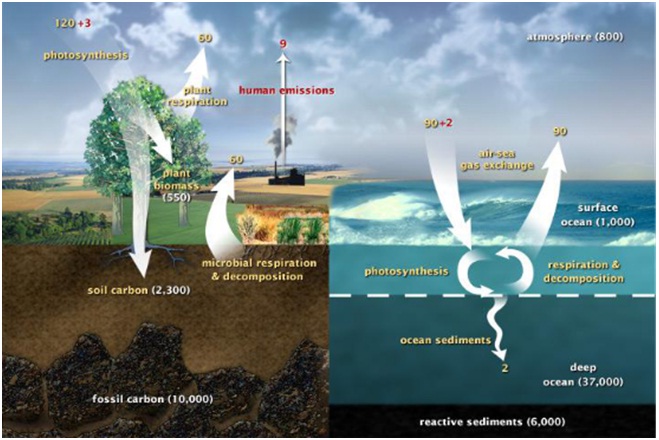
Since we were kids, we were all told in biology class that vegetation can absorb carbon dioxide from atmosphere, stored as organics and release oxygen through photosynthesis. In fact, there are other processes that we are not familiar with. The carbon which forest stored through photosynthesis is almost the same amount as those released by plant respiration, microbial respiration & decomposition in mature forests. Thus, forests may only work as carbon sink when they are in their growing stage (There is another theory that some mature forests start to work as sink again these years due to the carbon fertilization caused by greenhouse effect ). On the contrary, forest disturbance may release carbon from forest carbon pool to atmosphere, therefore aggregate greenhouse effect. So accurate estimation of forest biomass, hence carbon storage is of crucial importance to monitor carbon change dynamics. This knowledge will help us know how much carbon was released and how much can be restore in the future for better management.

What is Tree Biomass ?

Our fundamental knowledge of Forest AGB is based on destructive sampling in field, by choosing trees samples from different species, cutting them down, measuring tree metrics (normally tree height), diameter at breast height (DBH), weighing their dry weight in lab, then developing regression models between biomass and these metrics based on tree species. Finally these biomass models, normally as a function of DBH and tree height will be used to estimate biomass in larger area.

How Do We Monitor Biomass In a Large Scale in the Past?

Forest Inventory-Time & Money Consuming

Traditionally, extensive forest biomass estimation mainly rely on national forest inventory, gathering tree metrics (DBH, tree height etc.) for selected representative sites, which usually take years of time and large amount of manpower and money, not even to mention multi-temporal observation for change detection. And always, using small area to represent the whole picture can lead into bias.

Optical Remote Sensing – an Economical Way

The most mature and widely used technique is space-borne optical remotely sensing(Landsat, MODIS etc.). They can provide global seamless coverage repeatedly in a very short period.

However, signals optical images observe mostly reflected from surface of forests. These sensors can not provide vertical structure information which are more directly related to biomass and carbon storage. Also, they are very limited to weather conditions, which hindered its potential for accurate biomass estimation.

Microwave Remote Sensing – Better choice

Comparing with space-borne optical sensors, space-borne synthetic aperture radar (SAR) has stronger penetrating power, especially L-band and P-band signal with long wavelength can penetrate tree crown, bouncing from branches and tree trunks to receiver. These back scatters are related to vertical structure of forests, which can be used for canopy height hence biomass modeling (Ranson and Sun, 1994). However, the uncertainty of microwave remote sensing increases with the complexity of topography. Also, in dense forests, SAR back scatters can saturate easily. These limitations hindered its usage in large scale biomass mapping.

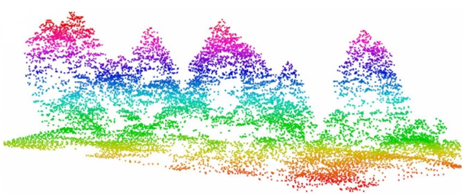
Airborne LIDAR – Accurate But Expensive

Light detection and ranging (LiDAR) can provide detailed information about 3D tree structure. It is by far the most accurate way to measure tree structural metrics, such as crown cover, tree height, canopy height and tree density. Has been widely used in regional forest above-ground biomass study and has been proved that biomass it estimated is closely related to field measurements. However the massive data volume and time and money consuming impede its usage in large area observation. The common method is to use airborne lidar systems as sampling method to extrapolate structural information and biomass against space-borne optical data set or space-borne SAR image which have complete coverage, which can also solve the scale mismatch problem between field measurement and space-borne data.

What Can Be Done in the Future?

Developing Accurate Species Specific Allometric Equations

Currently, forest biomass estimation in large scales mainly rely on general allometric equations developed from average conditions of many tree species as species specific allometric equations for many species simply do not exist, which would lead large uncertainty into the final results at the first place. In order to improve estimating accuracy in the future, species base allometric equations or more accurate general models should be developed.

Future Sensors

The new launched Sentinel-2 with its freely available multi-spectral data will be used in supporting forest monitoring, land cover change detection and natural disaster management. The first satellite, Sentinel-2A was lunched on 23 June 2015, and Sentinel-2B is planned to be lunched in mid of 2016. The Multi-Spectral Instrument (MSI) has 13 spectral bands from the visible to short-wave infrared(SWIR) with four at 10m, six at 20m and three at 60m resolution, with narrower bands and additional red channels compared to Landsat OLI for identification and assessing vegetation, and dedicated bands for improving atmospheric correction and detecting clouds(Drusch et al., 2012).

BIOMASS satellite with P-band (435Mhz, ~69m wavelength) will be launched by European Space Agency (ESA) in 2020 to generate 200 m resolution forest AGB map at global scale. Combining Airborne lidar measurements, initial tomographic phase using polarimetric SAR (PolSAR) images will be used to estimate forest AGB for low biomass areas, while in dense forests, PolInSAR phase will be used to extract tree height information and then convert to AGB using allometric equation derived from field measurements (Minh et al., 2016).

SAOCOM satellites (1A and 1B), both will be equipped with a L-band (about 1275 GHz) full polarimetric Synthetic Aperture Radar (SAR), the launch dates currently are scheduled on October 2017 and October 2018. And also a L-band (24-centimeter wavelength) polarimetric SAR   will be settled on NASA-ISRO SAR Mission (NISAR) schedule at 2019-2020.

A conceptual study of space-borne vegetation LiDAR called MOLI (Multi- Footprint Observation LiDAR and Imager) was conducted by Japan Aerospace Exploration Agency. If this plan finally settled, combining with airborne lidar, this will enable the appearance of the most accurate global biomass map.

Combination of Active and Passive Remote Sensing Observation

Combining different information extracted from multiple sensors will be the main trend for future above ground biomass estimation, such as combining space-borne optical multi-spectral data set and airborne hyperspectral, space-borne SAR and airborne lidar.

Modeling Biomass Using Non-parameter Machine Learning Models

The developing trend of modeling methods is a transfer from parameter methods like Multiple linear regression to complex machine learning models such as Decision tree, Artificial Neural Network (ANN), Support Vector Regression (SVR) etc.

References

DRUSCH, M., DEL BELLO, U., CARLIER, S., COLIN, O., FERNANDEZ, V., GASCON, F., HOERSCH, B., ISOLA, C., LABERINTI, P. & MARTIMORT, P. 2012. Sentinel-2: ESA’s optical high-resolution mission for GMES operational services. Remote Sensing of Environment, 120;25-36.

MINH, D. H. T., LE TOAN, T., ROCCA, F., TEBALDINI, S., VILLARD, L., RÉJOU-MÉCHAIN, M., PHILLIPS, O. L., FELDPAUSCH, T. R., DUBOIS-FERNANDEZ, P. & SCIPAL, K. 2016. SAR tomography for the retrieval of forest biomass and height: Cross-validation at two tropical forest sites in French Guiana. Remote Sensing of Environment, 175;138-147.

NIZAMI, S. MIRZA, & S. LIVESLEY. 2009. “Estimating carbon stocks in sub-tropical pine (Pinusrox burghii) forests of Pakistan,” Pak J AgriSci. Vol. 46(4)

RANSON, K. J. & SUN, G. 1994. Mapping biomass of a northern forest using multifrequency SAR data. Geoscience and Remote Sensing, IEEE Transactions on, 32; 388-396.

 

Time Terminologies: GMT and UTC

Although time terminologies are often spoken and used but still many of us do not have proper understanding of terms like GMT and UTC. Let us have a basic review of these terms.

GMT stands for Greenwich Mean Time (also called Meridian Time or Zulu Time) and it is a time standard since 1884. It was chosen because the Prime Meridian (the line of 0° Longitude) runs through Greenwich. Greenwich was a royal park and palace on a hill to the south of the River Thames east of London. Thus, Greenwich Mean Time (GMT) is the mean solar time at the Royal Observatory in Greenwich, London.

UTC is abbreviated from Coordinated Universal Time and it is The World’s Time Standard. Coordinated Universal Time (UTC) is the basis for civil time today. This 24-hour time standard is kept using highly precise atomic clocks combined with the Earth’s rotation.

UTC is the time standard commonly used across the world. The world’s timing centers have agreed to keep their time scales closely synchronized – or coordinated – therefore the name Coordinated Universal Time.

Two components are used to determine UTC:

• International Atomic Time (TAI): A time scale that combines the output of some 400 highly precise atomic clocks worldwide, and provides the exact speed for our clocks to tick.
• Universal Time (UT1), also known as astronomical time or solar time, refers to the Earth’s rotation. It is used to compare the pace provided by TAI with the actual length of a day on Earth.

GMT vs UTC

GMT is often interchanged or confused with UTC. But GMT is a time zone and UTC is a time standard.

Although GMT and UTC share the same current time in practice, there is a basic difference between the two:

• GMT is a time zone officially used in some European and African countries. The time can be displayed using both the 24-hour format (0 – 24) or the 12-hour format (1 – 12 am/pm).
• UTC is not a time zone, but a time standard that is the basis for civil time and time zones worldwide. This means that no country or territory officially uses UTC as a local time.

UTC does not changes with seasons. GMT was replaced with UTC as reference time scale on 1 January 1972. UTC or atomic time that include leap seconds, guaranteed to always be within 0.9 seconds of GMT.

UTC Zones (Source: http://www.jesusgilhernandez.com)

“Time Zone refers to any region where the same standard time is kept. It is one of more than 24 divisions of the earth, based on sections 7.5 degrees east and west of every 15 degree increment of longitude. There are 24 time zones (360 degrees divided by 15 degrees is 24) plus several offset time zones. Time zones allow the time to follow the rotation of the earth, providing a noon time at the approximate zenith of the sun in the sky of a given location.”

The local time within a time zone is defined by its offset (difference) from UTC, the world’s time standard. This offset is expressed as either UTC- or UTC+ and the number of hours and minutes.

UTC, GMT and Daylight Saving Time

“Daylight Saving Time (DST) is the practice of setting the clocks forward one hour from standard time during the summer months, and back again in the fall, in order to make better use of natural daylight.”

Neither UTC nor GMT ever change for Daylight Saving Time (DST). However, some of the countries that use GMT switch to different time zones during their DST period.

Daylight Time in Different Time Zones (Source: http://www.time.gove/)

For example, the United Kingdom is not on GMT all year, it uses British Summer Time (BST), which is one hour ahead of GMT, during the summer months.

Time Differences in Different Time Zones (Source: http://copradar.com)

Insight into the Maps

A map is a symbolic representation of selected characteristics of a place, usually drawn on a flat surface. Maps present information about the world in a simple, visual way. In order to understand maps properly, there are certain parameters which need to be understand thoroughly. Map scale is the most important parameter in all others.

Map Scale

Scale is defined as the ratio of the distance on a map to the corresponding distance on the surface the map represents. There are three forms of map scales i.e. Verbal Scale, Graphic or Bar Scale and Ratio or Representative Fraction (RF). Reader may explore further to understand these three terms thoroughly.

The Bar Scale is particularly important when enlarging or reducing maps by photocopy techniques because it changes with the map. If the Bar Scale is included in the photocopy, you will have an indication of the new scale.

Types of Scale

Very Important: – In order to use Ratio or RF, one must need to mention map size (A4 or A3 etc.) like in above figure A3 size is mentioned. It is very important to understand that an area shown on A3 size will have different Ratio when same areas is shown to A4 size map. Thus enlarging or reducing maps by photocopy techniques may add confusions in RF if map size is not mentioned on original map.

Small Tip: – It is a worthy practice to add both Bar Scale and Ratio on map for good understanding of readers

Conversion from one Form of Scale to Another

Units play an important role in order to convert scales from one form to another. Simple thing to remember is: ‘making units same’.

Here is an example of converting from Verbal Scale to RF. Remember, the RF has the same unit of measurement on both sides of the colon.

1 inch = 10 miles –> 1 inch = 10 x 63,360 inches (as 1 mile = 633,600 inches)

Thus RF= 1:633,600

To convert from RF to Verbal Scale you convert the fraction to familiar units of measurements; for example:

1:250,000 –> 1 inch equals 250,000 inches (63,360 inches = 1 mile)

Thus Verbal scale = 1 inch equals 4 miles

Small Scale and Large Scale Maps

These terms are often misinterpreted, a large scale map refers to one which shows greater detail and small scale map shows small detail. For simple understanding, a large scale map is a map which have a large Representative Fraction (RF) i.e. small denominator. For example, a map having ration or RF 1:10,000 = 1/10,000 is large scale map as compared to 1:500,000 = 1/500,000 scale map (small scale). General classification among different scales are given below

• Large Scale Maps: RF = 1:10,000 to 1:50,000
• Medium Scale Maps: RF = 1:50,000 to 1:250,000

• Small Scale Maps: RF = 1:250,000 to any denominator value greater than 250,000

Calculating Unknown Scale of a Map/Image

To calculate unknown scale by using a reference map or image with a known scale, locate two points on the reference map/image and the same two points on the map or photo of unknown scale. Measure this distance for both media and use the following formula to calculate the new scale:

S = UD / (RD * RS )

Where, S = Scale of the map or image which needs to be calculated

UD = Distance between the same two points measured from the map or image with unknown scale

RD = Distance between two points measured from the reference

RS = Scale of the reference map

For example, a topographic map at a scale of 1:100,000 can be used to determine the scale of a satellite image. In this case, two points are found which can be located in both the map and on the image. The distance between these two points on the topographic map is 12.7mm and the distance on the satellite image is 50.9mm. Entering this information in the formula, we have:

Satellite Image Scale = 50.9 / (12.7 * 1/100,000) = 1/24,951

To calculate scale using measurements in the field, measure the distance between two points in the field and measure the distance between the same two points in the map or image of unknown scale, Use the following formula to determine the scale of the map or image:

S = MD/RD

Where, S = Scale of the map or image which needs to be calculated

MD = Distance between the same two points measured from the map or image with the unknown scale

RD = Distance between two points measured in the field

Note: – The units of RD and MD must be the same.

For example, the scale of a satellite image can be determined using this technique by measuring the distance between two points on the satellite image and then measuring the distance between the same two points in the field. If, for example, the distance measured on the map was 50.9 mm and the distance in the field was 515 m (515000 mm) the scale can be calculated as follows:

Satellite Image Scale = 50.9 mm / 515,000 mm = 1/10,118

Map Scale and Raster Resolution

In 1987, Waldo Tobler, renowned analytical cartographer (now emeritus from University of California-Santa Barbara) wrote, “The rule is: divide the denominator of the map scale by 1,000 to get the detectable size in meters. The resolution is one half of this amount.”

Raster resolution (in meters) = Map Scale / 1000 /2

Map Scale vs Raster Resolution

For example, if you were not sure what resolution imagery you needed to acquire to detect features at a map scale of 1:50,000, using Tobler’s rule above, you can determine that imagery of approximately 25m [50000/ (1000*2)] resolution would be sufficient

Similarly, if you need to find out the mapping scale from a known imagery resolution you can do so using the formula below:

Map Scale = Raster resolution (in meters) * 2 * 1000

Here’s an example. Say you have a raster with a resolution of 30 meters. Each pixel is 30 meters on a size (an area of 900 square meters). You double that to get four pixels (two rows and two columns) with a resolution of 60 meters on a size (an area of 3600 square meters). Then you multiply that 60 meter resolution by 1000 to get a map scale of 60,000. (Source: ESRI).

Finding Feature’s Location Error w.r.t Ground Position on the Basis of Map Accuracy

Below is the formula to find feature’s location error

Feature’s location error = Map Accuracy * Map Scale

For example, a horizontal data are confidently positioned within 0.02″, at map scale, of the true ground position then for 100000 map scale

Feature location error = 0.02″ x 100,000 = 2000″ = 167 ft = 50 m

Similarly for 24000 scale, error = 0.02″ x 24,000 = 480″ = 40 ft = 12 m

Maps Scanning and DPI

Looking at dots per inch (DPI), it works just like architectural scale. The higher the scale we wish to achieve (say 200’=1″), the more feet we pack into one inch on paper. 400′ scale packs twice as many linear feet into one inch on paper as 200′ scale does.

If we have 200 feet per inch on a paper map, and we scan it at 200 dots per inch, then we get one foot per one dot. Each and every pixel of the computer-scanned image represents one foot on the map and in the real world.

UTM Zones and Pakistan

One can find a lot of literature on Universal Transverse Mercator (UTM), the Transverse Mercator projection is widely used around the world and works especially well for mapping areas smaller than a few degrees longitudinally, such as a state or county. It is based on 60 pre-defined standard zones to supply parameters. UTM zones are six degrees wide. Each zone exists in a North and South part of globe. Pakistan falls under northern zones of UTM i.e. 41N, 42N and 43N. Often, beginner level question is asked: what UTM zone is best suited for Pakistan? Well, a simple answer would be: it is based on the part of country we are considering, one may check zones allocation for Pakistan. Now, next question arises what if we use a UTM zone blindly? The answer is “Distortions”, there might be sever distortions/shifting in geographic features which can result “ill-mapping”. Below map shows what sort of distortion/shifting can occur at what area when different UTM zones are applied to the boundary of Pakistan.  We can clearly see that there is a shift in boundary towards north when we applied 42N and 43N zones for 41N region. Similar shift in 41N and 42N for 43N zone.  Why this happens? Because each UTM Zone is in fact a different projection using a different system of coordinates (local easting and northing for each zone). Thus in order to avoid such distortions, only a specified UTM zone should be applied for a specific area.

UTM Zones for Pakistan

Further clarification. . .

New users of UTM therefore will frequently attempt to “combine” different maps created in different UTM zones into one map with the expectation that the combined map will show all objects with low distortion as did the original maps. The motivating factor is often a desire to create a map centered on a region of interest that spans several UTM zones or which is centered between two zones. Such plans fail to take into account that UTM is an intrinsically inflexible system. In effect, the UTM system assumes objects from different zones will never be seen together in the same map.
Combining objects from different UTM zones into a map that is projected using only one of those UTM zones will result in distortion in the locations and shapes of the objects that originated in a different zone map. Geographic shapes that look good in a transverse Mercator projection centered upon a given UTM zone line will be very distorted when illustrated in a UTM projection centered upon a different zone line.
If we need to combine objects from several different UTM zones, the correct solution is to choose a different projection (such as a conic or azimuthal projection) for the combined map that provides low distortion over the entire region of interest. Remember, although no projection is perfect for all uses some projections are better than others in the uses for which they were designed. UTM was designed to map objects within one zone at a time. It is a very bad choice if objects from several zones must be shown together on the same map (source: http://www.georeference.org/)

Spatial, Geospatial and Geographic Data

These three are very relative terms often used interchangeably. We may not strict their usage but still there is a differentiation among these terms. After web surfing I found below text on these terms and it seems to be quite convincing.

The word spatial originated from Latin ‘spatium’, which means space. Spatial means ‘pertaining to space’ or ‘having to do with space, relating to space and the position, size, shape, etc.’ (Oxford Dictionary), which refers to features or phenomena distributed in three-dimensional space (any space, not only the Earth’s surface) and, thus, having physical, measurable dimensions. In GIS, ‘spatial’ is also referred to as ‘based on location on map’.

Geographic(al) means ‘pertaining to geography (the study of the surface of the earth)’ and ‘referring to or characteristic of a certain locality, especially in reference to its location in relation to other places’ (Macquarie Dictionary). Spatial has broader meaning, encompassing the term geographic. Geographic data can be defined as a class of spatial data in which the frame is the surface and/or near-surface of the Earth. ‘Geographic’ is the right word for graphic presentation (e.g., maps) of features and phenomena on or near the Earth’s surface. Geographic data uses different feature types (raster, points, lines, or polygons) to uniquely identify the location and/or the geographical boundaries of spatial (location based) entities that exist on the earth surface. Geographic data are a significant subset of spatial data, although the terms geographic, spatial, and geospatial are often used interchangeably.

Geospatial is another word, and might have originated in the industry to make the things differentiate from geography. Though this word is becoming popular, it has not been defined in any of the standard dictionary yet. Since ‘geo’ is from Greek ‘gaya’ meaning Earth, geospatial thus means earth-space. NASA says ‘geospatial means the distribution of something in a geographic sense; it refers to entities that can be located by some co-ordinate system’. Geospatial data is to develop information about features, objects, and classes on Earth’s surface and/or near Earth’s surface. Geospatial is that type of spatial data which is related to the Earth, but the terms spatial and geospatial are often used interchangeably. United States Geological Survey (USGS) says “the terms spatial and geospatial are equivalent”.

The concluded equation is:

spatial data > geospatial data == geographic data

(Source: Aragon at gis.stackexchange.com/)

Welcome

Welcome to Geospatial Club.